今回は、Googleが開発した人気の深層学習フレームワーク「TensorFlow」について、初心者にも分かりやすく解説します。TensorFlowの基本概念から実際の使い方まで、段階的に説明していきます。
動画で詳しく学習したい方はこちらもおすすめ
TensorFlowとは?
TensorFlowは、Googleが開発したオープンソースの機械学習・深層学習フレームワークです。2015年に公開されて以来、世界中の研究者や開発者に愛用されています。
TensorFlowの特徴
- 多様な用途:機械学習から深層学習まで幅広くカバー
- スケーラブル:スマートフォンからクラウドまで対応
- 豊富なエコシステム:TensorBoard、TensorFlow Lite、TensorFlow.jsなど
- 高い柔軟性:研究から本格的なプロダクション環境まで対応
なぜTensorFlowが人気なのか?
- Googleの強力なサポート:継続的な開発とアップデート
- 豊富なドキュメント:充実した学習リソース
- 活発なコミュニティ:世界中の開発者が情報共有
- 産業界での実績:多くの企業で実際に使用されている
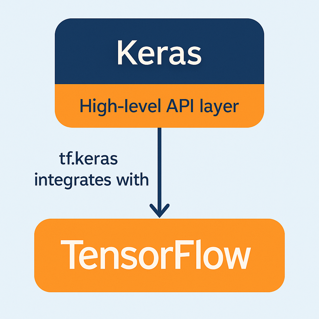
TensorFlowとKerasの関係
TensorFlowを語る上で欠かせないのがKerasとの関係です。
Kerasとは?
Kerasは、深層学習モデルを簡単に構築できる高レベルAPIです。TensorFlow 2.0以降、Kerasはtf.kerasとしてTensorFlowに統合されました。
# TensorFlow 2.x以降の書き方
import tensorflow as tf
from tensorflow import keras

# モデル構築
model = tf.keras.Sequential([
    tf.keras.layers.Dense(128, activation='relu'),
    tf.keras.layers.Dense(10, activation='softmax')
])
TensorFlowとKerasの使い分け
- tf.keras:初心者や素早いプロトタイピングに最適
- 低レベルAPI:研究や複雑なカスタマイズが必要な場合
- 実際の開発:多くの場合tf.kerasで十分
TensorFlowのインストール
必要な環境
TensorFlowを使用するには以下の環境が必要です:
- Python 3.7-3.11
- pip 19.0以降
- 64bit版のPython
インストール方法
# CPU版のインストール
pip install tensorflow

# GPU版を使用する場合(CUDA対応グラフィックカード必要)
pip install tensorflow-gpu
インストール確認
import tensorflow as tf

# TensorFlowのバージョン確認
print(f"TensorFlow version: {tf.__version__}")

# GPU利用可能か確認
print(f"GPU available: {tf.config.list_physical_devices('GPU')}")
TensorFlowの基本概念
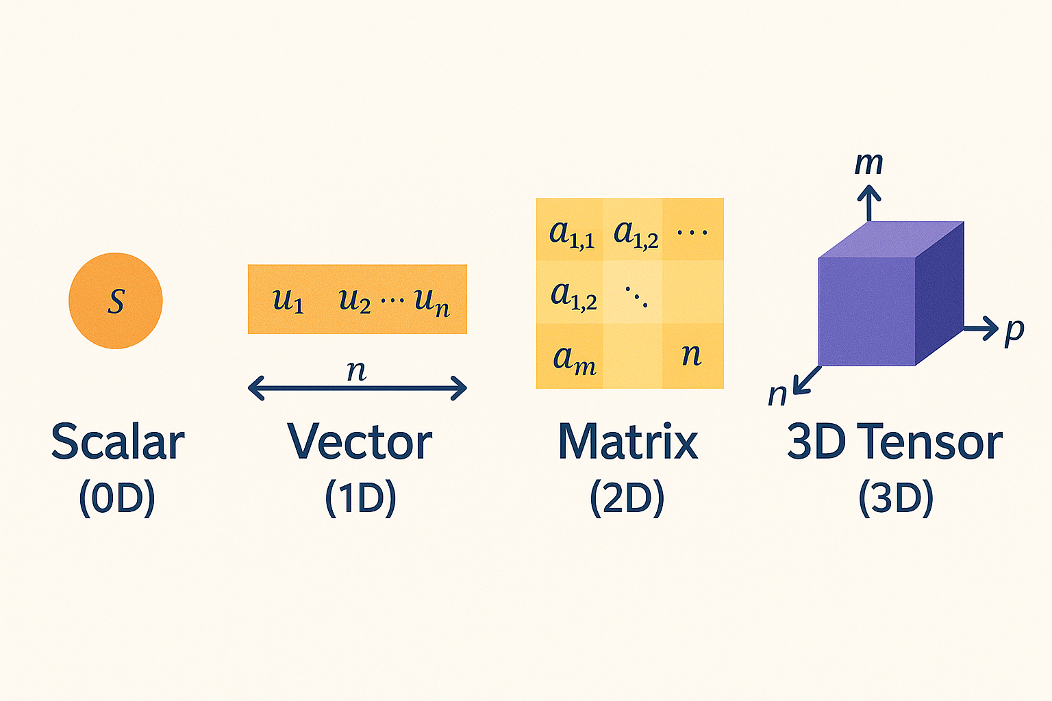
1. テンソル(Tensor)
テンソルは、TensorFlowの基本的なデータ構造です。多次元配列として考えることができます。
import tensorflow as tf

# スカラー(0次元テンソル)
scalar = tf.constant(42)
print(f"スカラー: {scalar}")

# ベクトル(1次元テンソル)
vector = tf.constant([1, 2, 3, 4])
print(f"ベクトル: {vector}")

# 行列(2次元テンソル)
matrix = tf.constant([[1, 2], [3, 4]])
print(f"行列:\n{matrix}")

# 3次元テンソル
tensor_3d = tf.constant([[[1, 2], [3, 4]], [[5, 6], [7, 8]]])
print(f"3次元テンソル:\n{tensor_3d}")
2. データ型と形状
# テンソルの情報を確認
matrix = tf.constant([[1.0, 2.0], [3.0, 4.0]])

print(f"データ型: {matrix.dtype}")      # float32
print(f"形状: {matrix.shape}")          # (2, 2)
print(f"次元数: {matrix.ndim}")         # 2
print(f"要素数: {tf.size(matrix)}")     # 4
3. 基本的な演算
# テンソルの基本演算
a = tf.constant([[1, 2], [3, 4]])
b = tf.constant([[5, 6], [7, 8]])

# 要素ごとの演算
print(f"加算: \n{tf.add(a, b)}")
print(f"乗算: \n{tf.multiply(a, b)}")

# 行列積
print(f"行列積: \n{tf.matmul(a, b)}")

# 数学関数
c = tf.constant([1.0, 4.0, 9.0])
print(f"平方根: {tf.sqrt(c)}")
print(f"対数: {tf.math.log(c)}")
実践!最初のニューラルネットワーク
1. データセットの準備
MNISTデータセット(手書き数字)を使用して、実際にニューラルネットワークを構築してみましょう。
import tensorflow as tf
from tensorflow import keras
import numpy as np
import matplotlib.pyplot as plt

# MNISTデータセットの読み込み
(x_train, y_train), (x_test, y_test) = keras.datasets.mnist.load_data()

print(f"訓練データの形状: {x_train.shape}")
print(f"テストデータの形状: {x_test.shape}")
print(f"ラベルの種類: {np.unique(y_train)}")

# データの可視化
plt.figure(figsize=(10, 2))
for i in range(5):
    plt.subplot(1, 5, i+1)
    plt.imshow(x_train[i], cmap='gray')
    plt.title(f'Label: {y_train[i]}')
    plt.axis('off')
plt.show()
2. データの前処理
# データの正規化(0-255 → 0-1)
x_train = x_train.astype('float32') / 255.0
x_test = x_test.astype('float32') / 255.0

# データの形状変換(28x28 → 784)
x_train = x_train.reshape(-1, 28 * 28)
x_test = x_test.reshape(-1, 28 * 28)

print(f"前処理後の訓練データ形状: {x_train.shape}")
print(f"前処理後のテストデータ形状: {x_test.shape}")
3. モデルの構築
# Sequential APIを使用したモデル構築
model = tf.keras.Sequential([
    # 入力層(784次元)
    tf.keras.layers.Dense(128, activation='relu', input_shape=(784,)),

    # ドロップアウト層(過学習防止)
    tf.keras.layers.Dropout(0.2),

    # 隠れ層
    tf.keras.layers.Dense(64, activation='relu'),

    # 出力層(10クラス分類)
    tf.keras.layers.Dense(10, activation='softmax')
])

# モデルの概要表示
model.summary()
4. モデルのコンパイル
# 最適化手法、損失関数、評価指標の設定
model.compile(
    optimizer='adam',                    # 最適化手法
    loss='sparse_categorical_crossentropy',  # 損失関数
    metrics=['accuracy']                 # 評価指標
)
5. モデルの訓練
# モデルの訓練
history = model.fit(
    x_train, y_train,
    epochs=10,              # エポック数
    batch_size=128,         # バッチサイズ
    validation_split=0.2,   # 検証データの割合
    verbose=1               # 進捗表示
)
6. モデルの評価
# テストデータでの評価
test_loss, test_accuracy = model.evaluate(x_test, y_test, verbose=0)
print(f"テスト精度: {test_accuracy:.4f}")

# 学習曲線の可視化
plt.figure(figsize=(12, 4))

plt.subplot(1, 2, 1)
plt.plot(history.history['loss'], label='Training Loss')
plt.plot(history.history['val_loss'], label='Validation Loss')
plt.title('Model Loss')
plt.xlabel('Epoch')
plt.ylabel('Loss')
plt.legend()

plt.subplot(1, 2, 2)
plt.plot(history.history['accuracy'], label='Training Accuracy')
plt.plot(history.history['val_accuracy'], label='Validation Accuracy')
plt.title('Model Accuracy')
plt.xlabel('Epoch')
plt.ylabel('Accuracy')
plt.legend()

plt.tight_layout()
plt.show()
7. 予測の実行
# 予測の実行
predictions = model.predict(x_test[:5])

# 結果の可視化
plt.figure(figsize=(15, 3))
for i in range(5):
    plt.subplot(1, 5, i+1)
    plt.imshow(x_test[i].reshape(28, 28), cmap='gray')

    # 予測確率が最も高いクラス
    predicted_class = np.argmax(predictions[i])
    confidence = np.max(predictions[i])

    plt.title(f'予測: {predicted_class}\n信頼度: {confidence:.2f}')
    plt.axis('off')
plt.show()
TensorFlowの高度な機能
1. Functional API
より複雑なモデルを構築する場合は、Functional APIを使用します。
# Functional APIによるモデル構築
inputs = tf.keras.Input(shape=(784,))
x = tf.keras.layers.Dense(128, activation='relu')(inputs)
x = tf.keras.layers.Dropout(0.2)(x)
x = tf.keras.layers.Dense(64, activation='relu')(x)
outputs = tf.keras.layers.Dense(10, activation='softmax')(x)

functional_model = tf.keras.Model(inputs=inputs, outputs=outputs)
functional_model.summary()
2. カスタムレイヤー
# カスタムレイヤーの作成
class CustomDenseLayer(tf.keras.layers.Layer):
    def __init__(self, units):
        super(CustomDenseLayer, self).__init__()
        self.units = units

    def build(self, input_shape):
        self.w = self.add_weight(
            shape=(input_shape[-1], self.units),
            initializer='random_normal',
            trainable=True
        )
        self.b = self.add_weight(
            shape=(self.units,),
            initializer='zeros',
            trainable=True
        )

    def call(self, inputs):
        return tf.matmul(inputs, self.w) + self.b

# カスタムレイヤーの使用
custom_model = tf.keras.Sequential([
    CustomDenseLayer(128),
    tf.keras.layers.Activation('relu'),
    tf.keras.layers.Dense(10, activation='softmax')
])
3. コールバック関数
# コールバック関数の設定
callbacks = [
    # 早期終了
    tf.keras.callbacks.EarlyStopping(
        monitor='val_loss',
        patience=3,
        restore_best_weights=True
    ),

    # 学習率の調整
    tf.keras.callbacks.ReduceLROnPlateau(
        monitor='val_loss',
        factor=0.5,
        patience=2,
        min_lr=1e-7
    ),

    # モデルの保存
    tf.keras.callbacks.ModelCheckpoint(
        'best_model.h5',
        monitor='val_accuracy',
        save_best_only=True
    )
]

# コールバック付きで訓練
model.fit(
    x_train, y_train,
    epochs=50,
    batch_size=128,
    validation_split=0.2,
    callbacks=callbacks
)
TensorFlowエコシステム
1. TensorBoard
TensorBoardは、TensorFlowの可視化ツールです。
# TensorBoardログの設定
import datetime

log_dir = "logs/fit/" + datetime.datetime.now().strftime("%Y%m%d-%H%M%S")
tensorboard_callback = tf.keras.callbacks.TensorBoard(
    log_dir=log_dir,
    histogram_freq=1
)

# TensorBoard付きで訓練
model.fit(
    x_train, y_train,
    epochs=10,
    validation_split=0.2,
    callbacks=[tensorboard_callback]
)

# TensorBoardの起動(ターミナルで実行)
# tensorboard --logdir logs/fit
2. TensorFlow Lite
モバイルデバイス向けの軽量化されたモデルを作成できます。
# TensorFlow Liteモデルへの変換
converter = tf.lite.TFLiteConverter.from_keras_model(model)
tflite_model = converter.convert()

# モデルの保存
with open('model.tflite', 'wb') as f:
    f.write(tflite_model)

print("TensorFlow Liteモデルが保存されました")
3. TensorFlow Serving
本格的なプロダクション環境でのモデル配信に使用されます。
# SavedModel形式での保存
model.save('saved_model/my_model')

# モデルの読み込み
loaded_model = tf.keras.models.load_model('saved_model/my_model')
TensorFlowのベストプラクティス
1. データパイプラインの最適化
# tf.dataを使用した効率的なデータパイプライン
def create_dataset(x, y, batch_size=128):
    dataset = tf.data.Dataset.from_tensor_slices((x, y))
    dataset = dataset.shuffle(buffer_size=1000)
    dataset = dataset.batch(batch_size)
    dataset = dataset.prefetch(tf.data.AUTOTUNE)
    return dataset

train_dataset = create_dataset(x_train, y_train)
test_dataset = create_dataset(x_test, y_test)

# データセットを使用した訓練
model.fit(train_dataset, epochs=10, validation_data=test_dataset)
2. Mixed Precision
GPU使用時の高速化とメモリ使用量削減に効果的です。
# Mixed Precisionの有効化
policy = tf.keras.mixed_precision.Policy('mixed_float16')
tf.keras.mixed_precision.set_global_policy(policy)

# モデル構築時の注意点
model = tf.keras.Sequential([
    tf.keras.layers.Dense(128, activation='relu'),
    tf.keras.layers.Dense(64, activation='relu'),
    # 出力層はfloat32で計算
    tf.keras.layers.Dense(10, activation='softmax', dtype='float32')
])
3. グラフ実行の活用
# @tf.functionデコレータによる高速化
@tf.function
def train_step(x, y):
    with tf.GradientTape() as tape:
        predictions = model(x, training=True)
        loss = loss_function(y, predictions)

    gradients = tape.gradient(loss, model.trainable_variables)
    optimizer.apply_gradients(zip(gradients, model.trainable_variables))
    return loss
他の深層学習フレームワークとの比較
TensorFlow vs PyTorch
| 特徴 | TensorFlow | PyTorch |
|---|---|---|
| 学習曲線 | やや急 | 比較的緩やか |
| デバッグ | TensorBoard | シンプル |
| プロダクション | 強い | 改善中 |
| 研究用途 | 普通 | 人気 |
| コミュニティ | 大きい | 成長中 |
どちらを選ぶべきか?
- TensorFlow:プロダクション重視、エコシステム活用
- PyTorch:研究開発、プロトタイピング重視
よくある問題と解決方法
1. メモリ不足エラー
# GPU メモリの制限設定
gpus = tf.config.experimental.list_physical_devices('GPU')
if gpus:
    try:
        for gpu in gpus:
            tf.config.experimental.set_memory_growth(gpu, True)
    except RuntimeError as e:
        print(e)
2. 学習が進まない場合
# 学習率の調整
initial_learning_rate = 0.001
lr_schedule = tf.keras.optimizers.schedules.ExponentialDecay(
    initial_learning_rate,
    decay_steps=1000,
    decay_rate=0.96,
    staircase=True
)

optimizer = tf.keras.optimizers.Adam(learning_rate=lr_schedule)
3. 過学習の対策
# 正則化手法の組み合わせ
model = tf.keras.Sequential([
    tf.keras.layers.Dense(128, activation='relu'),
    tf.keras.layers.BatchNormalization(),
    tf.keras.layers.Dropout(0.3),

    tf.keras.layers.Dense(64, activation='relu'),
    tf.keras.layers.BatchNormalization(),
    tf.keras.layers.Dropout(0.3),

    tf.keras.layers.Dense(10, activation='softmax')
])
次のステップ
実践プロジェクト
- 画像分類:花の種類分類、猫犬判別
- 自然言語処理:感情分析、文章生成
- 時系列予測:株価予測、気温予測
- 画像生成:GANを使った画像生成
まとめ
今回は、TensorFlowの基本から実践的な使い方まで解説しました。
重要なポイント
- TensorFlowは Google 開発の強力な深層学習フレームワーク
- tf.kerasにより初心者でも使いやすくなった
- 豊富なエコシステムでプロダクション環境まで対応
- 段階的な学習で着実にスキルアップが可能
TensorFlowは最初は複雑に感じるかもしれませんが、基本概念を理解すれば強力なツールとして活用できます。まずは簡単なプロジェクトから始めて、徐々に複雑なモデルに挑戦してみてください。
次回は、畳み込みニューラルネットワーク(CNN)を使った画像認識について詳しく解説予定です。